
Predicting Malignancy in Breast Tumours Using a SVM
Summary
This project develops a Support Vector Machine (SVM) classification model to predict whether breast tumours are benign or malignant using digitized image measurements. The final classifier achieved strong performance on the held-out test set, correctly classifying 104 of 109 cases. However, the model produced one false negative—misclassifying a malignant tumour as benign—which is clinically critical because it could delay diagnosis and treatment. The results show that while an SVM can provide useful decision support for screening and flagging high-risk cases, careful calibration and further refinement are required before relying on it in real-world clinical workflows.
Introduction
Breast cancer remains one of the most prevalent cancers among women, with early detection shown to dramatically improve outcomes. Patients diagnosed at early stages have a 5-year survival rate of 99%, compared to only 31% for late-stage diagnoses. Traditional tumour diagnosis methods can be subjective and depend heavily on physician experience.
An accurate machine learning classifier could provide several benefits:
- Objectivity: Reducing subjectivity in diagnosis by providing consistent, data-driven predictions
- Scalability: Enabling more efficient screening programs in resource-limited settings
- Early intervention: Supporting faster diagnostic pathways to improve patient outcomes
- Clinical decision support: Assisting physicians by flagging high-risk cases for additional review
Since benign tumours tend to remain localized while malignant tumours can invade surrounding tissue and metastasize, accurate classification is critical for determining appropriate treatment and follow-up. A well-calibrated machine learning model will not replace clinical judgment, but it can support physicians by highlighting patterns that might be missed at scale and by flagging cases that merit closer review.
Research Question
Can we build a machine learning model to accurately predict whether a newly discovered breast tumour is benign or malignant based on digitized image measurements of tumour cell nuclei?
Methods
All data manipulation and analysis was performed in Python using pandas for data wrangling, NumPy for numerical computing, scikit-learn for machine learning, and Altair for visualization. The computational environment was containerized with Docker to ensure reproducibility across different systems.
Data
The Wisconsin Diagnostic Breast Cancer (WDBC) dataset was retrieved from the UCI Machine Learning Repository. Created by Dr. William H. Wolberg, W. Nick Street, and Olvi L. Mangasarian at the University of Wisconsin-Madison, the dataset contains measurements computed from digitized images of fine needle aspirate (FNA) samples of breast masses.
The dataset consists of:
- 569 instances (357 benign, 212 malignant)
- 30 real-valued features representing measurements of cell nuclei characteristics
- 1 binary target variable (Diagnosis: Benign or Malignant)
Each feature represents one of ten cell nucleus characteristics (radius, texture, perimeter, area, smoothness, compactness, concavity, concave points, symmetry, and fractal dimension) computed in three forms:
- Mean value across cells
- Standard error (SE) of the values
- Maximum ("worst") value observed
Feature Analysis
Distribution Analysis
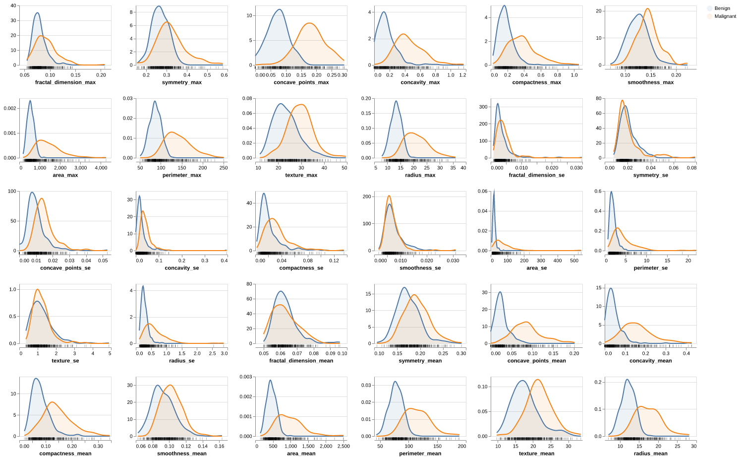
Figure 1: Distribution Analysis. Distribution of all 30 features colored by diagnosis class. Size-related features (radius_mean, perimeter_mean, area_mean) show clear separation between benign (blue) and malignant (orange) tumours, with malignant tumours exhibiting consistently larger values. Shape complexity features (concavity_mean, concave_points_mean) demonstrate strong discriminative power, with malignant tumours showing higher irregularity. Texture and smoothness features display substantial overlap between classes, suggesting lower individual predictive value. Right skewness is evident in area and concavity features, particularly in their standard error (_se) variants.
Outlier Analysis
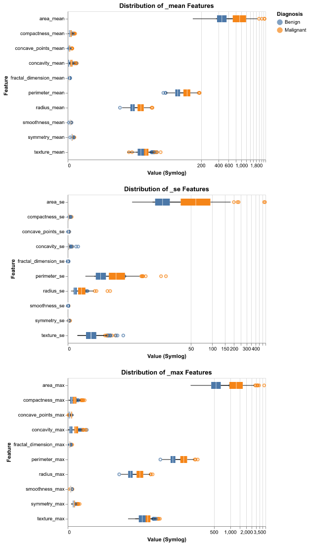
Figure 2: Looking at Outliers. Numerous outliers were observed, particularly in malignant samples for size-related features. These extreme values are not data errors but represent biologically meaningful signals characteristic of aggressive tumour growth. Therefore, these outliers were retained in the analysis as they contain critical diagnostic information.
Correlation Analysis
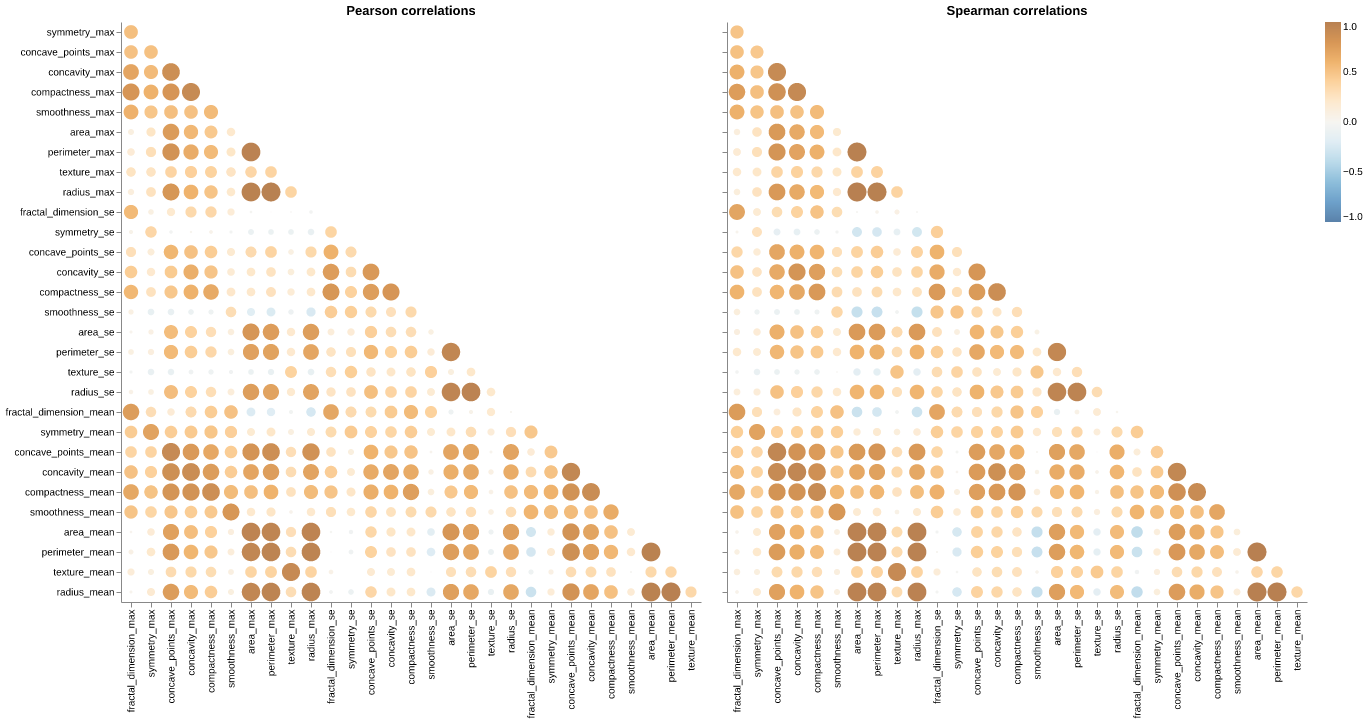
Figure 3: Multicollinearity. Pearson and Spearman correlation matrices revealing severe multicollinearity. Near-perfect correlation (r > 0.95) between radius, perimeter, and area across all three statistical forms (_mean, _se, _max). Strong positive correlations (r > 0.85) among concavity, concave_points, and compactness. Similar correlation patterns observed in both Pearson (linear) and Spearman (monotonic) metrics. This multicollinearity is geometrically expected but creates redundancy that can destabilize models and inflate variance.
Pairwise Separability
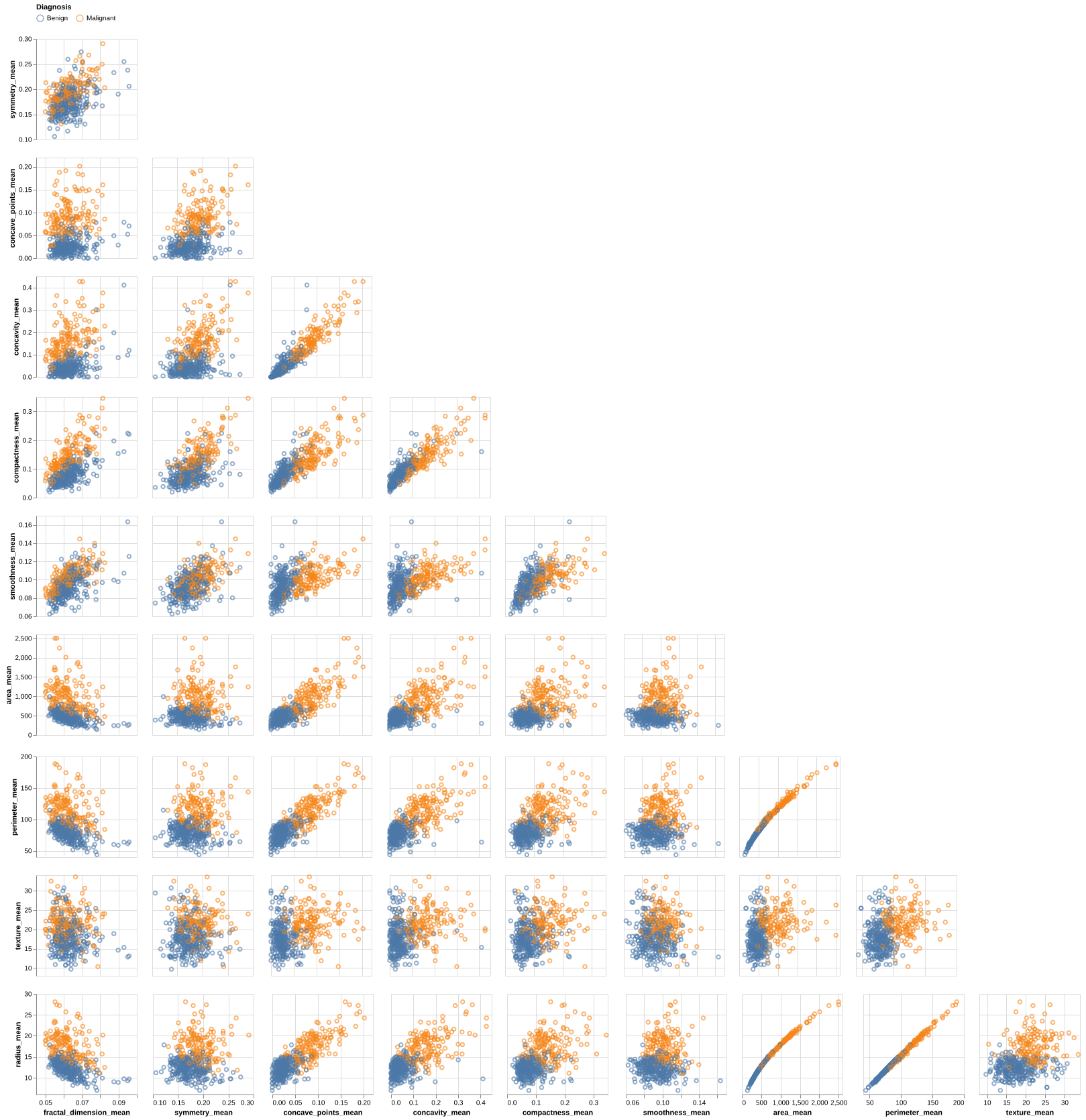
Figure 4: Pairwise Separability. Pairplot visualizing 2D relationships between selected features. Size-related features (radius_mean, area_mean) combined with shape complexity metrics (concavity_mean, concave_points_mean) demonstrate clear class separation with minimal overlap. The curved relationship between area and radius reinforces the geometric redundancy identified in correlation analysis.
Initial Findings
- Class Separation:
- High Separability: Features related to size (radius, perimeter, area) and concavity (concave_points, concavity) show clear distinction between Benign and Malignant classes (Malignant samples generally have higher values).
- Low Separability: Texture, Smoothness, and Fractal Dimension show significant overlap, indicating they are weaker individual predictors.
- Distributions:
- Skewness: "Area" and "Concavity" features (both _mean and _se) are heavily right-skewed.
- Outliers: Visible in the upper tails of area_max and perimeter_se.
- Correlations (Multicollinearity):
- Severe Multicollinearity: radius, perimeter, and area are highly correlated. This is expected geometrically but redundant for models.
- concavity, concave_points, and compactness also exhibit very high positive correlation.
Preprocessing Pipeline
Based on the initial exploratory analysis, the following steps were implemented in the modeling pipeline:
- Feature Selection: We removed redundant features to reduce multicollinearity.
- Scaling: Since our features vary vastly in scale (e.g., area > 1000 vs. smoothness < 0.2), we used StandardScaler to standardize all features to unit variance.
Model Development
A Support Vector Machine (SVM) classifier with radial basis function (RBF) kernel was selected. SVM was chosen because:
- It performs well on high-dimensional data
- It is effective with clear class separation as observed in our initial feature analysis
Hyperparameter Tuning
Grid search with 15-fold cross-validation was performed to optimize:
- C (regularization parameter): [0.001, 0.01, 0.1, 1.0, 10.0, 100.0]
- gamma (kernel coefficient): [0.001, 0.01, 0.1, 1.0, 10.0, 100.0]

Figure 5: Heatmap for SVM GridSearchCV Mean Test Score. The heatmap shows mean test scores across the hyperparameter grid. The optimal hyperparameters were C = 10.0 and gamma = 0.001. These values provided the best balance between model complexity and generalization performance, achieving the highest mean cross-validation score.
Results & Discussion
Model Performance
The final SVM classifier demonstrated strong performance on the test set while also revealing important trade-offs for clinical use. Figure 6 presents the confusion matrix, showing:
- True Negatives (Benign correctly classified): 68 cases
- False Positives (Benign misclassified as Malignant): 4 cases
- False Negatives (Malignant misclassified as Benign): 1 case
- True Positives (Malignant correctly classified): 41 cases
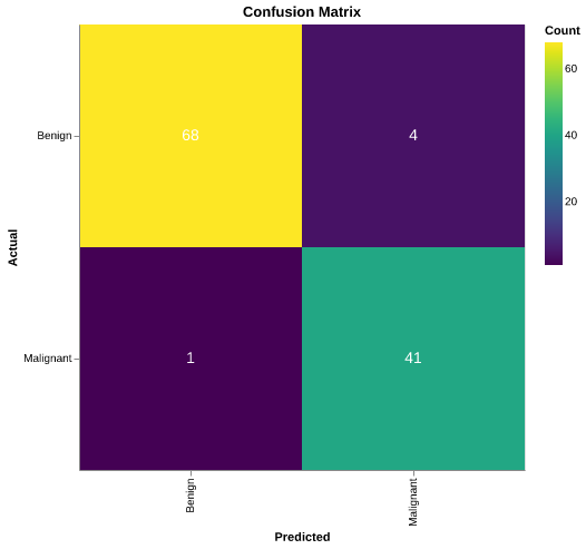
Figure 6: Heatmap for Confusion Matrix. The confusion matrix shows 68 true negatives, 4 false positives, 1 false negative, and 41 true positives. Overall test accuracy: 95.61% (109 correct predictions out of 114 test samples).
Overall test accuracy: 95.61% (109 correct predictions out of 114 test samples), which aligns with expectations given the clear separation observed in the size- and shape-related features during exploration.
From a purely statistical perspective, this is a high-performing classifier. From a clinical perspective, however, the single false negative stands out: even one missed malignant case in a small test set signals that, at scale, the model could still fail on patients where early intervention is most important. This tension between accuracy and clinical risk is central to how such models should be evaluated and deployed.
However, the presence of one false negative represents the primary concern. In a clinical context, false negatives are significantly more harmful than false positives. A false negative could lead to:
- Delayed diagnosis and treatment initiation
- Disease progression to more advanced, less treatable stages
- Reduced survival probability
Moreover, while the four false positives (benign tumours classified as malignant) are less critical as they are likely to lead to follow-up testing rather than immediate treatment, they still represent unnecessary patient anxiety and healthcare costs.
Clinical Implications
The model's 96% accuracy is promising but insufficient for clinical deployment as a standalone diagnostic tool. Medical applications typically prioritize very high sensitivity for malignant cases to minimize false negatives, even at the cost of more false positives. The single false negative in this small test set suggests that at larger scale, the model could miss a non-trivial number of malignant cases if used without additional safeguards.
Limitations
Several limitations affect the interpretation of these results:
- Small test set: With only 114 test samples, performance estimates have wide confidence intervals
- Single dataset source: Model generalizability to other populations or imaging equipment is unknown
- Feature engineering: Limited exploration of feature interactions or polynomial features
Future Work
To improve model reliability for clinical use, we recommend:
- Class weight adjustment: Increase the penalty for false negatives during training to prioritize recall over precision
- Ensemble methods: Combine multiple classifiers to improve robustness
- External validation: Test on independent datasets from different medical centers to assess generalizability
- Feature engineering: Explore interaction terms and domain-specific features to capture complex patterns
- Error analysis: Conduct detailed investigation of misclassified cases to identify systematic patterns